Pre-Asymptotic Dispersion

Using age to resolve a longstanding critique of pre-asymptotic dispersion.  Intermittent flow in pipe networks and many other industrial and environmental fluid mechanical scenarios gives rise to transport of disinfectants and other solutes that are not described by the usual advection-dispersion equation with constant dispersion coefficient.  In many cases, including flow in pipes, the way that the dispersion coefficient changes with time since onset of flow is known and expressed by a mathematical equation (in e.g., Poisueille flow when pipe flow is laminar).  Classically this challenge is handled by expressing the dispersion coefficient as a function of time.  But in the case where solutes are continuously entering the flow system, as in the case of disinfectant solutes entering a building from a water main, this gives rise to overlapping solutes (due to dispersion) with multiply-defined values of the dispersion coefficient.  This problem was explicitly called out by G.I. Taylor (Taylor, G. I., 1959, The present position in the theory of turbulent diffusion.  Adv Geophysics 6:101–112).

Given the intermittent nature of flows in premise plumbing pipe networks, it can be expected that transport of disinfectants etc. is essentially always under the pre-asymptotic regime, while period of stagnation lead to increased overlap of solutes by diffusion along a pipe.  Thus it is necessary to resolve Taylor’s critique of the classical method in order to develop a mathematical modeling technology for handling pre-asymptotic dispersion during intermittent flows in pipe networks.  We have addressed this using age, interpreted similarly as in subsection b.).  In our pipe network model of subsection b.), age is the total age of the water or solute to the pipe network regardless of whether the water is flowing or not.  Here we apply ageing only when the water is flowing, so that the water age represents cumulative time of exposure of the water to the flowing condition.  For reference, the classical advection-dispersion equation with constant dispersion coefficient is

where c is the solute concentration, v is the velocity, and D is the dispersion coefficient. Our version including age to flow conditions is

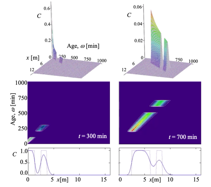
Where is the on-off switch for ageing to flow, which takes on the value of unity when the water is flowing and zero when it is stagnant, and where ω  is age.  This second form leads to the solute concentration becoming a function of age-to-flowing-conditions, ω, as in c = c(t, ω, x) and the usual measurable solute concentration is the integral of c(t, ω, x) over age.  We have developed both the mathematical properties of this new approach, two remarkably simple closed-form solutions to classical boundary- and initial-value problems, and a numerical approach to solution of this second equation in order to generate solutions to advective-dispersive transport of solutes under pre-asymptotic conditions.  

Transport of solutes in flowing fluid involves only advection and diffusion. Because one cannot characterize all the variations in fluid velocity at small scales, when modeling transport at larger scales we manufacture an upscaled transport flux that is supposed to account for these variations, called dispersion, with classical models of dispersion adopted from Fick’s law of diffusion, with varying degrees of success in representing averaged concentrations. However this approach requires solutes to experience the full range of velocity variations before this (“asymptotic”) Fickian model can work. In many cases of environmental fluid mechanics this experience takes such a long time that so-called “preasymptotic” dispersion conditions prevail. Prior efforts to model preasymptotic dispersion involve making the dispersion coefficient a function of time-since-injection or of distance-transported, in bulk fluids and in groundwater. This approach is critiqued G. I. Taylor who created the concept of asymptotic dispersion because it requires multiply-defined dispersion coefficients for solutes injected at different start times but which overlap due to dispersive spreading.  We resolve this problem by using residence-time (“age”) as the independent variable for the dispersion coefficient.