Under Construction… still

Exposure-time in Fluid Mechanics

The concept of exposure-time is a generalization of “age” – when one component of a flow is exposed to another, one can keep track of the associated exposure-time by literally moving the exposed component in a new dimension added to the governing equations of transport. Here are two examples, from a ppt deck on this approach (56.2Mb, got movies, also links to papers).

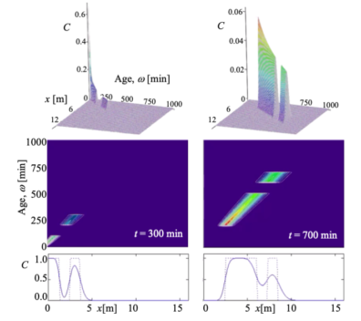
Transient groundwater age in a vertical 2D section of aquifer. The red box is a 2D vertical cross-section of an aquifer with no-flow boundaries on left and bottom, and sinusoidally varying pressure gradient on top (seasonal flow forcing). By adding an age dimension (“y”, shown in the movie) along which we advect water at unit velocity we add a “clock” to the governing equation and can visualize age as a distribution along y at any point (x, z) in the aquifer.  An application of this approach to regional groundwater flow is here.


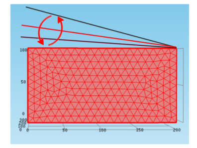
Scalar Dissipation. The insert shows particles in a 2D shear flow including a dispersing solute cloud. We use the same clock approach but now with age in the vertical direction and advect particles at velocity proportional to the magnitude of the gradient of solute in the horizontal plane.  The movie shows the evolution of the age as the cumulative exposure of solute particles to scalar dissipation which is a proxy for mixing and for reaction extent.

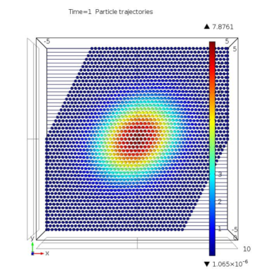
Multidomain Diffusion

When a mobile fluid is in contact with a material that allows only diffusive transport, there occurs diffusive exchange between the mobile phase and the diffusive “immobile” phase.  The diffusive exchange adds extraordinarily long residence times to the transport through such materials.  Examples include transport in: fractured and porous material, groundwater in a porous medium with low-conductivity inclusions or even microscopically-permeable solid phases, river corridors with exchange between river and sediment bed domains, pipes lined with biofilms, gas phases over the ocean or lakes, as well as biological, industrial, and chemical engineering applications.  Mathematical modeling of such exchange has a rich history starting apparently with Carslaw and Jaeger in transport and Villermaux in chromatography, leading to the general “Memory function” form for such exchange.  Memory function models encapsulate a wide range of models used not only for mobile-immobile exchange but also so-called anomalous dispersion or non-Fickian transport (multirate mass transfer, time-fractional advective-dispersive transport, and many continuous-time random walk models).  However, the memory function operator induces anomalous delays (and not anomalous transport) which when coupled with conventional transport model operations can give rise to arbitrarily specified (e.g., power-law) tailing.
All memory function models can be cast as first-order exchange models where the rate of immobile-mobile zone exchange depends on time spent in the immobile zone.  Such a “phase exposure-dependent exchange” (PhEDExWRR2017) model is used here to simulate a groundwater injection/withdrawal experiment reported in Gouze et al. (2008).

Pre-asymptotic dispersion

Transport of solutes in flowing fluid involves only advection and diffusion. Because one cannot characterize all the variations in fluid velocity at small scales, when modeling transport at larger scales we manufacture an upscaled transport flux that is supposed to account for these variations, called dispersion, with classical models of dispersion adopted from Fick’s law of diffusion, with varying degrees of success in representing averaged concentrations. However this approach requires solutes to experience the full range of velocity variations before this (“asymptotic”) Fickian model can work. In many cases of environmental fluid mechanics this experience takes such a long time that so-called “preasymptotic” dispersion conditions prevail. Prior efforts to model preasymptotic dispersion involve making the dispersion coefficient a function of time-since-injection or of distance-transported, in bulk fluids and in groundwater. This approach is critiqued G. I. Taylor who created the concept of asymptotic dispersion because it requires multiply-defined dispersion coefficients for solutes injected at different start times but which overlap due to dispersive spreading.  We resolve this problem by using residence-time (“age”) as the independent variable for the dispersion coefficient.
The figure shows profiles at two times for 1D transport of two sequential injected solute pulses in a 16 m long flow at constant velocity of 12 cm/min and dispersion coefficient that relaxes exponentially to an asymptotic value of 12 cm^2/min.  The dispersive flux causes overlap of the two pulses in space, but this poses no problem when the dispersion coefficient is a function of the solute age.


Reactive Transport

River corridors, aquifers, pipe networks, etc. are flow domains in which multicomponent suspended or dissolved substances undergo multiple biogeochemical reactions, some fast. We work on the formulation and solution of mathematical models that honor the important processes despite upscaling to develop simplified and practical models. Current focus is on distinguishing true mixing from dispersive spreading and on generalized modeling of diffusive exchange between mobile and immobile phases..
~
Details, papers.