The most updated lab writing instructional modules are available: engineeringlabwriting.org
Learning Objectives
This module is designed to assist engineering instructors in strengthening lab instruction materials so that students should be able to:
- Explain how error propogates or compounds in computations involving random variables.
- Use a rule of thumb to estimate the error in computed results.
- Calculate the error in a result computed using products or quotients.
Why Should Students Care About Propagation of Error?
In experimental work, increasing confidence in measured results is important because too much error or uncertainty in a result can render that result useless. Experiments fraught with error are not valuable, but error is inevitable, so both quantifying error and reducing it becomes very important. Computations are often made using values that have error due to measurement precision and other uncertainty. Offering a reader the error bounds for a result that is computed from measured values provides valuable information about the quality of the computed result.
How to Estimate Error in Computed Results
Estimating error is better than not considering error at all. Because engineers are masters of heuristics (tools that use time-saving simplifying assumptions), we will first introduce an easy way to estimate error. The error in any computed result, expressed as a percentage, must be greater than the individual error of any input value and is less than the summation of individual errors in all input values. The error in the computed result is closer to the value of the largest error in the input values. There is usually one measurement in any experiment with the greatest error that dominates the error in the computed result.
How to Rigorously Calculate Error in Computed Results
Propagation of error depends on the mathematical operations performed on input values as well as their standard deviation (s). While calculating error propagation can be relatively complex, if two variables (A and B) are multiplied or divided and their errors are not correlated (meaning the errors are not related in some meaningful way) their standard deviations (SA and SB) are related to the standard deviation (Sf) of their product (ƒ=AB) or dividend (ƒ=A/B) by Equation 1.
![]()
If we assume we are working with normal distributions and 3s error bounds, then we can calculate error in a computed result given errors in input values using this procedure:
- Start with input value uncertainties (A ± 3sA), either as absolute values or relative percentages.
- Divide input values uncertainties by 3 to determine their standard deviations (sA).
- Relate those standard deviations to the standard deviation of the computed result (sƒ) using Equation 1.
- Determine the error in the computed result (3sƒ) and report the computed result with its uncertainty expressed as a percentage ƒ ± (3sƒ/ƒ)100%.
An Example of Error Eropagation
A common task in engineering materials and mechanics courses is to calculate the modulus of elasticity, E, a measure of material stiffness, of a specimen from a tension test involving
- Applied axial force, F.
- Deforming length of a specimen, L.
- Cross-sectional area of the specimen, A.
- The amount of stretch in the specimen between the unloaded and loaded states, ∆.
The relationship of the quantities to determine the modulus of elasticity is E=σ/ε = (F/A)/(∆/L), where σ is engineering stress (F/A) and ε is engineering strain (∆/L).
Taking a very simplified approach so we can focus on the propagation of error, we will examine a specimen of 6061-T6 aluminum load in its elastic range. The test depicted in Figure 1.
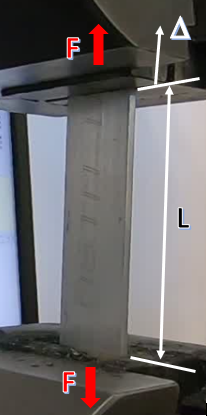
Figure 1. 6061-T6 aluminum sample in tensile tester, with force, deforming length, and stretch denoted.
Let us consider the error in the cross-sectional area of the specimen if its width and thickness are measured as 2.000 in. and 0.125 in., respectively with a measurement precision of 0.001 in. each. The 3s percent error is 0.80% for the thickness and 0.05% for the width. We assume the 0.001 in. is a 3s error, so the standard deviation is 0.001/3, or 0.00033 in. Using Equation 1 to calculate the standard deviation of the cross-sectional area, we determine
![]()
The absolute error is then 3sƒ or 0.002 in. 2, which is 0.80% of the 0.25-in.2 result. These calculations can be summarized in Table 1. It is worth noting that the relative error (%) in the cross-sectional area is equal to the relative error in the thickness measurement, because the measurement with the greatest error contributes the most significantly to the error in the computed result. It is also worth nothing that the relative error for the thickness measurement is greater than that for the width measurement because we are using the measurement device at the low end of its range. Relative error is reduced, in general, when using a measurement device at the high end of its range, because precision does not generally degrade within the working range of an instrument.
Table 1. Results of a cross-sectional area calculation including propagation of error
| Variable | Value | Std. Dev. | 3s absolute | 3s % |
|---|---|---|---|---|
| t (in.) | 0.125 | 0.000333 | 0.001 | 0.80% |
| w (in.) | 2.000 | 0.000333 | 0.001 | 0.05% |
| A (in.2) | 0.25 | 0.000668 | 0.0020 | 0.80% |
Now that we see how to calculate compounding error through a calculation involving a product of two values, let us perform these same calculations for the value of interest: modulus of elasticity.
Let’s say each input quantity has its own error based on measurement precision or uncertainty:
- the amount of force applied, F, is 1,000 lb and the resolution of the measurement is 5 lb or 0.5%.
- the deforming length, L, is 4 in. and the resolution of its measurement plus uncertainty based on potential deformation in the grips is relatively poor at 0.4 in. or 10.0%.
- the cross-sectional area, A, was computed above to be 0.25 in. 2 with a measurement precision of 0.002 in.2 or 0.8%.
- the stretch, ∆, measured when the load is applied is 0.0015 in. with a measurement precision of 0.0001 in. or 6.7%.
Using Equation 1 to calculate the standard deviation for computed results,
- the error in F is 0.5% and in A is 0.8%, so the error in the stress, σ=F/A, is 0.9%.
- the error in ∆ is 6.7% and in L is 10.0%, so the error in the strain, ε=∆/L, is 12.0%.
- the error in E=σ/ε is 12.1%, due primarily to the errors in strain resulting from the limit in the measurement precision of stretch, ∆, and uncertainty in the deforming length, L.
Table 2. Results of a modulus of elasticity calculation including propagation of error
| Variable | Value | Std. Dev. | 3s absolute | 3s % |
|---|---|---|---|---|
| F (lb) | 1,000 | 1.666667 | 5 | 0.50% |
| L (in.) | 4 | 0.133333 | 0.4 | 10.0% |
| ∆ (in.) | 0.0015 | 3.33E-05 | 0.0001 | 6.7% |
| A (in.2) | 0.25 | 0.000667 | 0.002 | 0.80% |
| σ=F/A (psi) | 4,000 | 12.57 | 37.73 | 0.9% |
| ε=∆/L (in./in.) | 0.000375 | 1.5E-05 | 4.51E-05 | 12.0% |
| E=σ/ε (psi) | 10,666,667 | 428,639 | 1,285,917 | 12.1% |
If we compute E, the result is 10,666,667 psi, or 10,667 ksi. We can calculate the error in E as ± 12.1% or ± 1,286 ksi. Therefore, the result E is actually somewhere between 9,381 ksi and 11,953 ksi.
The nominal value of modulus of elasticity published for 6061-T6 aluminum is 10,000 ksi. If an error analysis were not conducted, the result of this experiment, 10,667 ksi, would appear to be in error or somehow inconsistent with the 10,000-ksi nominal value. One might compute the percent difference of the experimental value relative to the nominal value and report a 6.67% relative difference.
When accounting for error in the computed result, it can simply be concluded that the modulus of elasticity of the aluminum specimen is somewhere between 9,381 ksi and 11,952 ksi, which is consistent with published values.
If we had used the simplifying assumption of the most significant error in any input value to estimate the error in the modulus of elasticity, we would use the 10% of 10,667 ksi or ± 1,067 ksi, for a range of 9,600-11,734 ksi/ This much simpler analysis still confirms that the tested specimen has a stiffness consistent with the published nominal value, at least within our ability to measure this value.
These calculations are provided in a spreadsheet available here: Propagation of Error Example.
Common Mistakes by Students
- Error or uncertainty in computed results is not offered or considered.
- Excessive precision for a computed result is reported that indicates greater knowledge of the result than is possible (e.g. 4.14375 lb).
- An experimental result is compared to a published or expected value without considering error.
Where can I find tools to calculate the error in computed results?